Resources
- https://www.youtube.com/watch?v=kMNSAhsyiDg
- https://www.youtube.com/watch?v=b6xeOLjeKs0
- https://www.youtube.com/watch?v=Q4LYys9v9Ko
- https://www.youtube.com/watch?v=RRsq9apr5QY
- https://www.youtube.com/watch?v=Q4LYys9v9Ko - Tech Talk: What’s that Sound? An Overview of Shazam’s Audio Search Algorithm
- https://www.youtube.com/watch?v=LZ7THTB88AE - Cameron Macleod - Implementing a Sound Identifier in Python
- https://www.cameronmacleod.com/blog/how-does-shazam-work
- https://github.com/worldveil/dejavu
- https://www.youtube.com/watch?v=WhXgpkQ8E-Q - PWLTO#11 – Peter Sobot on An Industrial-Strength Audio Search Algorithm
- https://github.com/itspoma/audio-fingerprint-identifying-python
Audio Features Invariant to Signal Degradations
- fourier coefficients
- mel frequency cepstral coefficients (MFCC)
- spectral flatness
- sharpness
- linear predictive coding (LPC)
In order to extract a 32-bit frame, 33 non-overlapping frequency bands are selected
- frequency range from 300Hz to 2000Hz
- logarithmic spacing (HAS operates on approximately logarithmic bands)
Initial
yt-dlp -x "https://www.youtube.com/watch?v=hLQl3WQQoQ0"
ffmpeg -i song-01.opus -c:a pcm_s24le song-01.wav
import os
import librosa.display
import matplotlib.pyplot as plt
import numpy as np
audio_fpath = "./audio/"
audio_clips = os.listdir(audio_fpath)
# x, sr = librosa.load(audio_fpath + audio_clips[0], sr=None, offset=15.0, duration=0.01)
x, sr = librosa.load(audio_fpath + audio_clips[0], sr=None)
# x is the audio time series
# sr is the sample rate
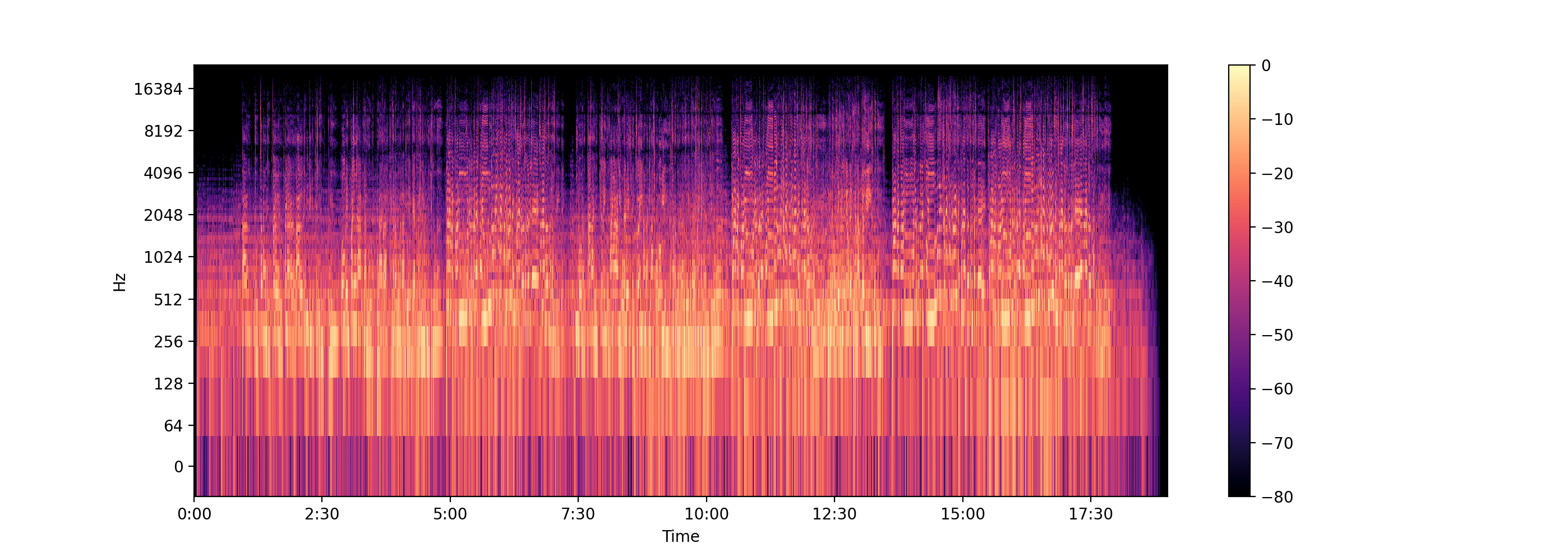
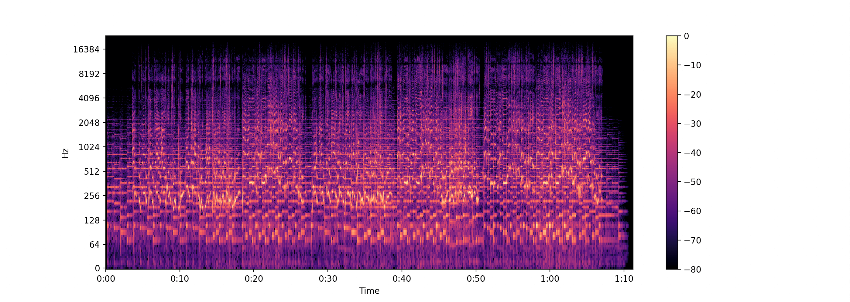
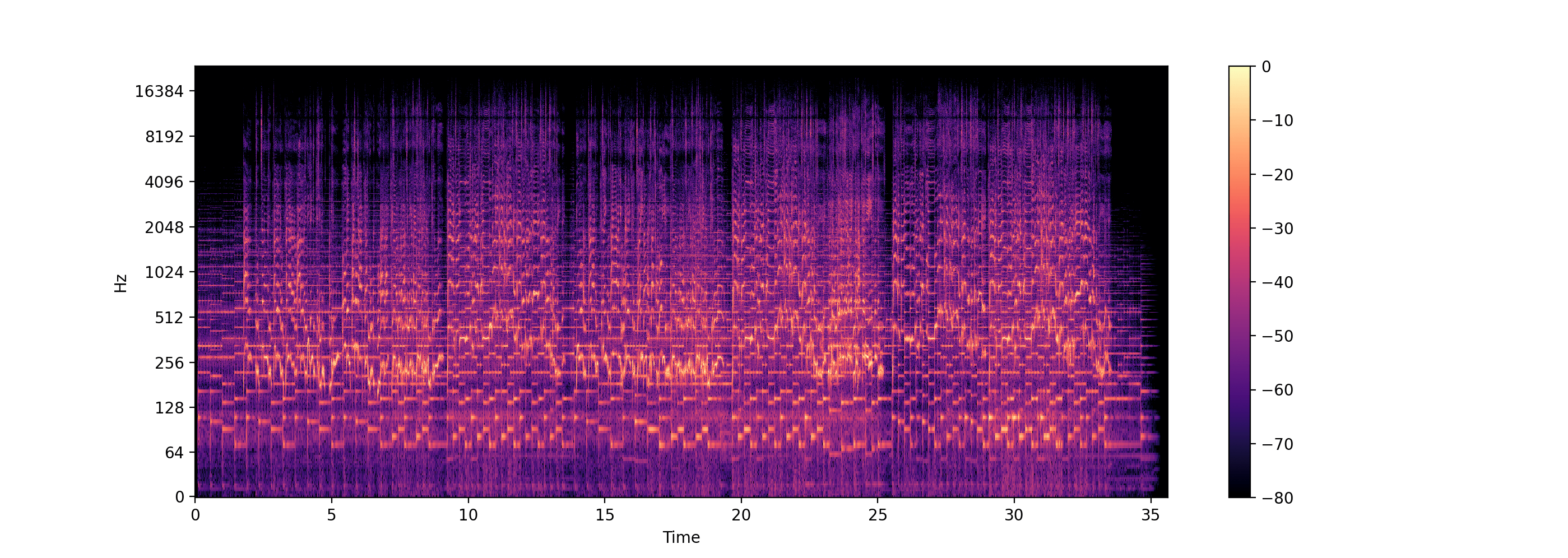
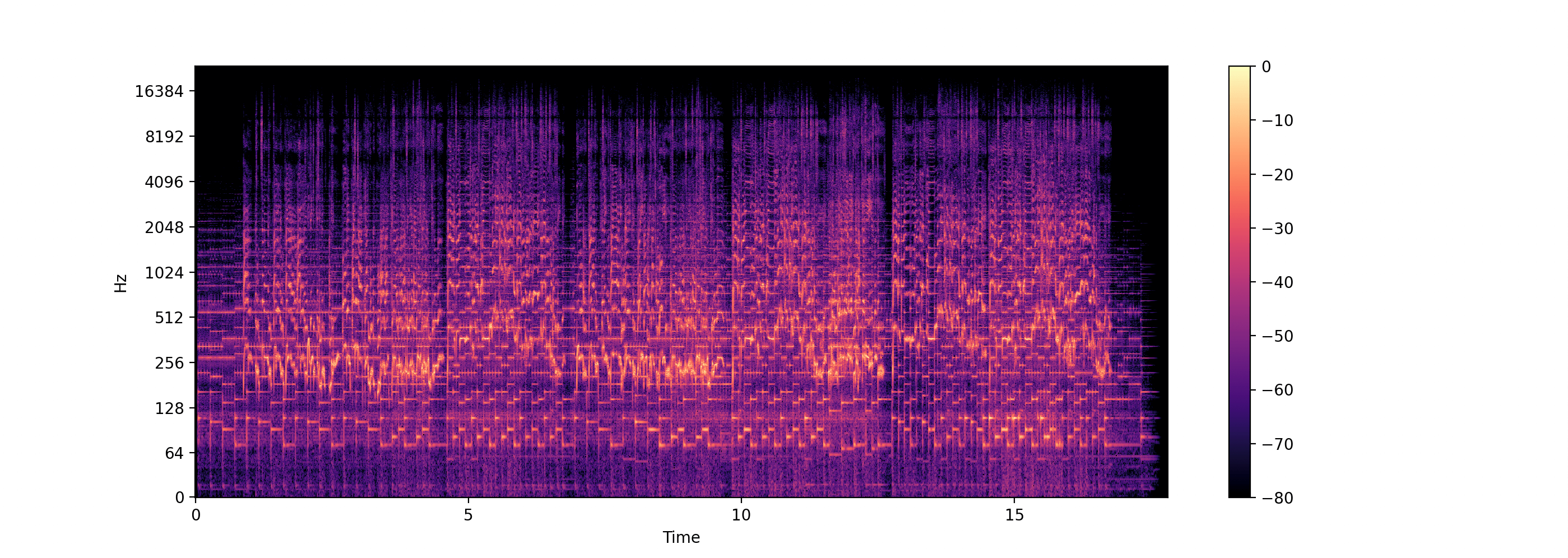
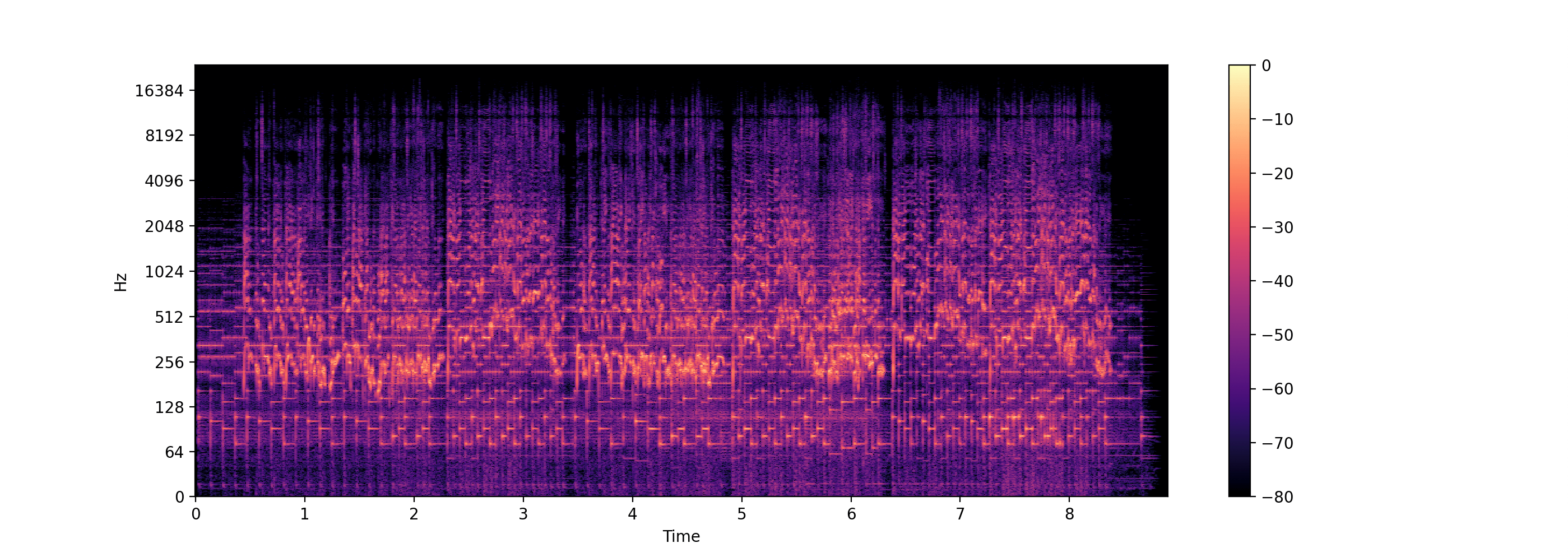
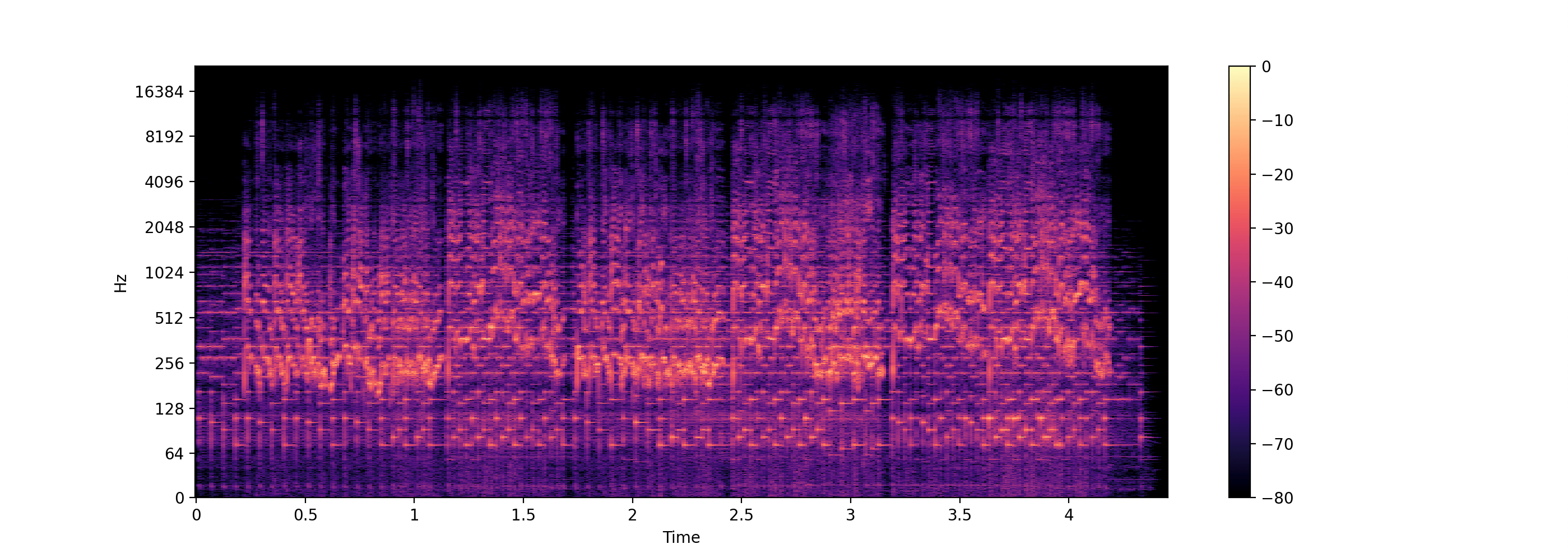
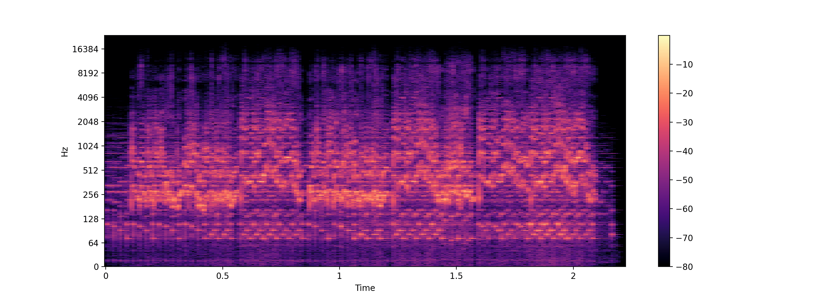
# Compute the Short-Time Fourier Transform (STFT)
D = librosa.stft(x, n_fft=131072)
D = np.abs(D)
# Convert amplitude to decibels (log scale)
log_D = librosa.amplitude_to_db(D, ref=np.max)
# Plot the log spectrogram
plt.figure(figsize=(14, 5))
librosa.display.specshow(log_D, sr=sr, x_axis='time', y_axis='log')
plt.colorbar()
plt.show()