Probability Density Distribution vs Probability Mass Distribution
Let’s say we have some function 𝑓(𝑥) that we haven’t named yet but we know that 𝑎∫𝑏𝑓(𝑥)𝑑𝑥 yields the probability that we see an outcome between 𝑎 and 𝑏. What should we call 𝑓(𝑥)? Well, what are its properties? Let’s start with its units. We know that, in general, the units on a definite integral 𝑎∫𝑏𝑓(𝑥)𝑑𝑥 are the units of 𝑓(𝑥) times the units of 𝑑𝑥. In our setting, the integral gives a probability, and 𝑑𝑥 has units in say, length. So the units of 𝑓(𝑥) must be probability per unit length. This means that 𝑓(𝑥) must be telling us something about how much probability is concentrated per unit length near 𝑥; i.e., how dense the probability is near 𝑥. So it makes sense to call 𝑓(𝑥) a “probability density function.” (In fact, one way to view 𝑎∫𝑏𝑓(𝑥)𝑑𝑥 is that, if 𝑓(𝑥) ≥ 0, 𝑓(𝑥) is always a density function. From this point of view, height is area density, area is volume density, speed is distance density, etc. One of my colleagues uses an approach like this when he discusses applications of integration in second-semester calculus.)
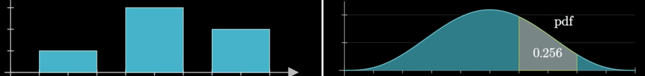
Now that we’ve named 𝑓(𝑥) a density function, what should we call the corresponding function in the discrete setting? It’s not a density function; its units are probability rather than probability per unit length. So what is it? Well, when we say “density” without a qualifier we are normally talking about “mass density,” and when we integrate a density function over an object we obtain the mass of that object. With this in mind, the relationship between the probability function in the continuous setting to that of the probability function in the discrete setting is exactly that of density to mass. So “probability mass function” is a natural term to grab to apply to the corresponding discrete function.
|
1 = 𝛴𝑥∊𝑋𝐏(𝑋=𝑥) |
1 = ∫𝑋𝑓(𝑥)𝑑𝑥 |
|
| |